VNA Calibration, Characterization and Uncertainties

While messing around with the HP 8720A I discovered a great free (for non commercial use) tool called METAS VNA Tools. This software suite offers a comprehensive array of tools for tracking various uncertainty contributors to VNA (Vector Network Analyzer) measurements. Among the most prominent contributors are:

• The VNA itself, encompassing factors such as drift, linearity error, power error, and noise floor.
• Cables, which influence phase stability and reflection stability.
• Connectors, where considerations include mating stability between different connector types (with further details pending).

My understanding of these topics has been greatly enhanced through insights gleaned from the METAS VNA Tools Google Groups[1], the manual for METAS VNA Tools[2] and the EURAMET (European Association of National Metrology Institutes) guide on VNA calibration[3]. These resources collectively offer a wealth of knowledge essential for optimizing VNA measurements and ensuring precision in metrology applications

Uncertainty contributors

Noise Floor, Trace Noise and Dynamic Range

The dynamic range of a network analyzer refers to the range between its maximum and minimum measurable values with accuracy. This critical metric is influenced by various factors:

• Averaging Factor
• Bandwidth of intermediate frequency
• Characteristics of the VNA itself, including its architecture, the type of reflection bridges used, and the performance of its receivers and power detectors.

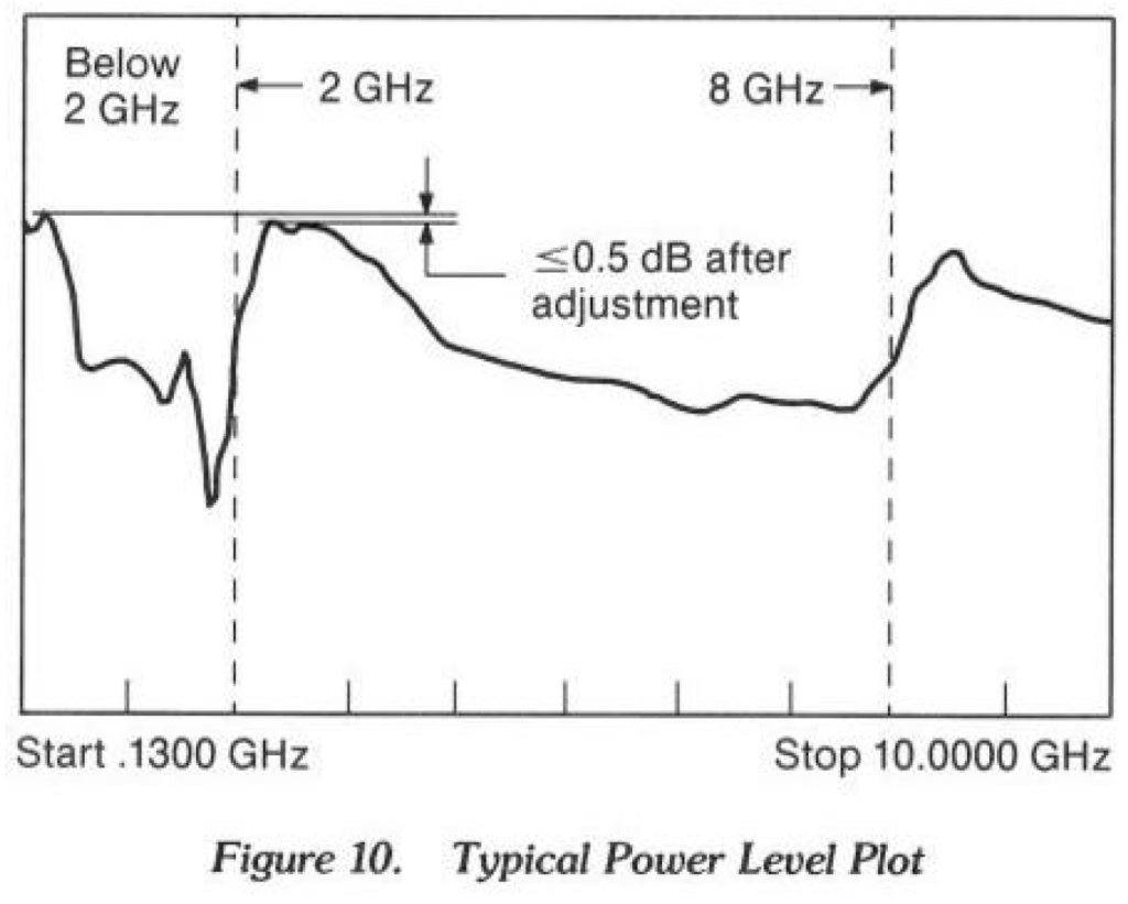
For instance, the user guide for the HP 8720A provides a practical example to illustrate this concept. Suppose the analyzer offers a bandpass with a stop band rejection of 70dB and has a maximum output power of -10 dBm. In such a scenario, achieving a noise floor below -80 dBm is necessary to meet the 70dB stop band rejection test criteria effectively.

Understanding and optimizing the dynamic range is crucial for accurate and reliable measurements in network analysis, ensuring that the analyzer can effectively capture signals across a wide range of amplitudes while maintaining precision and fidelity.

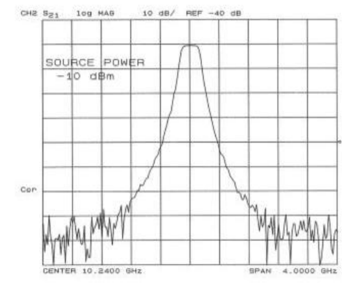
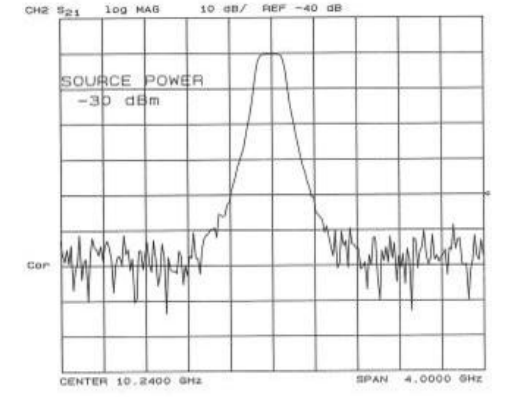
Shown by adjusting the output power from -10 dBm to -30 dBm which results in 20 dB worse signal to noise ratio. Pictures from the operating manual[4].

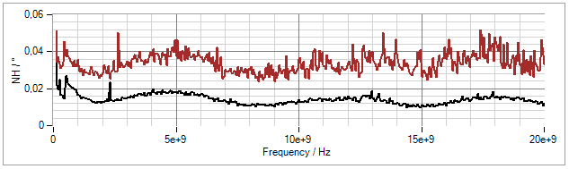
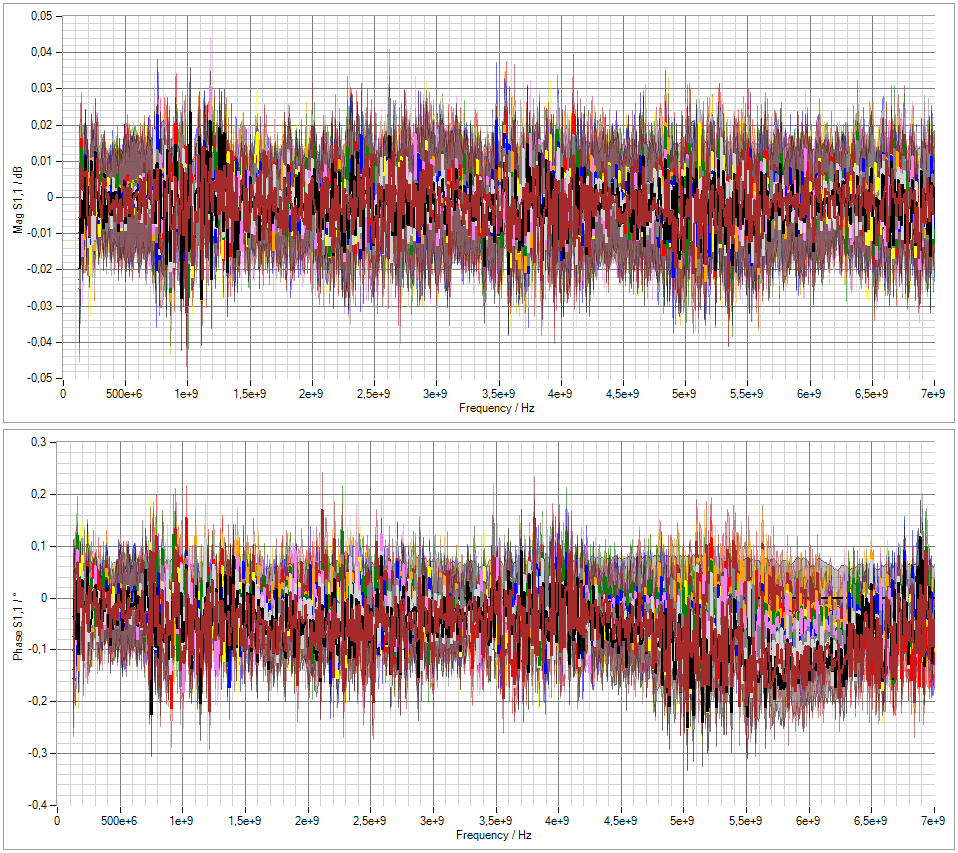
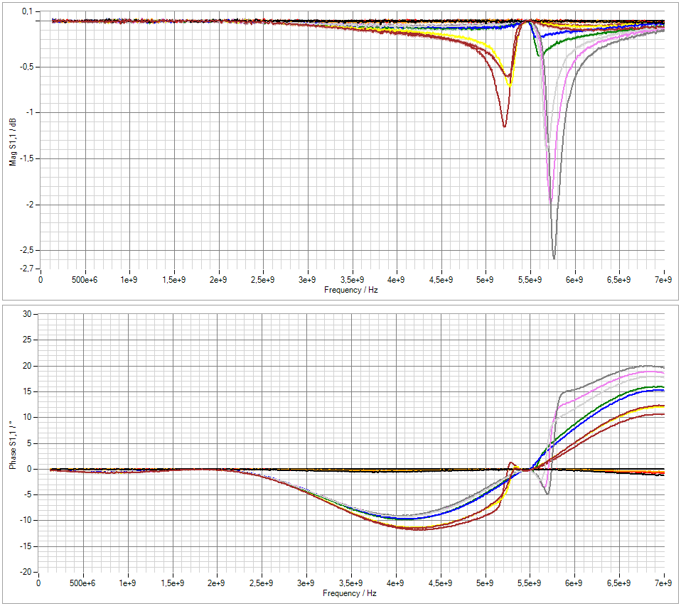
The implications of the IF bandwidths can be seen in the following graphs:

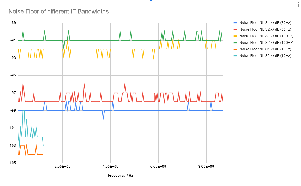
A tenth of the IF bandwidth results in approximately 10 dB better noise floor. Similar results can be achieved with sweep-to-sweep averaging. Generally there are different arguments for and against using the one or the other. Reducing the IF bandwidth – therefore digitally narrwoing the bandwidth of the receiver – of the VNA allows to see the response of the DUT after the first sweep and allows for better feedback in case something around the DUT has to be tuned (Antennas, Filters, etc…). IF bandwidth reduction also supresses spurs and harmonics way better than averaging, whilest averaging can reduce extreme low frequency noise way better. Both attenuate line noise quite well.

About my VNA specifically: The graph also shows definitly a difference between port 1 and port 2. Similiar behaviour can be observed when further down judging about the trace noise. I so far can not explain the difference with anything else than a defect of some sort.

Drift

To assess the drift of your VNA within its operating environment, a comprehensive approach typically involves conducting a full 2-Port calibration. Subsequently, measurements are taken to determine the maximum deviation of each succeeding measurement relative to the initial one obtained post-calibration. Various S-Parameters are of interest in this analysis and can be converted into deviations related to Symmetry, Tracking, Match, Directivity, Isolation, and Switch Terms.

The standard measurement setup entails conducting measurements on all calibration standards, followed by 96 measurements of all S-Parameters for a thru connection. These measurements are spaced at intervals of 15 minutes over a total duration of 24 hours.

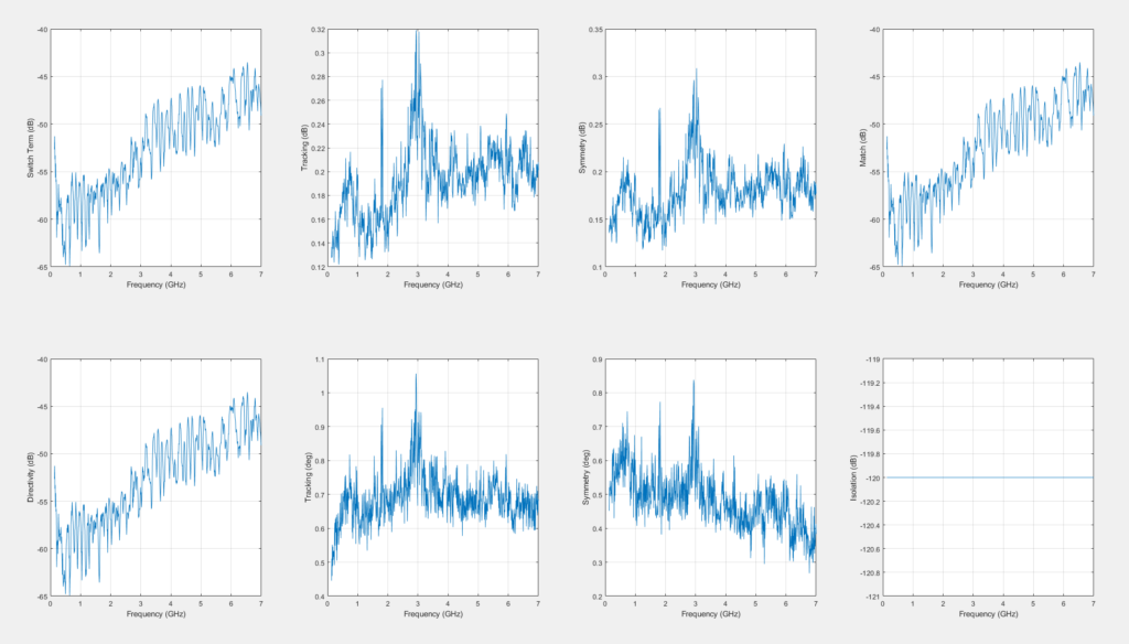
The measurement above was executed with the help of the measurement series (Drift specialization) of the METAS VNA Tools and the drifts were determined with a Matlab Script which post processes these measurements[5].

Linearity

As – nearly – every measurement device is the VNA is also susceptible to linearity errors in general. The approach mentioned by the EURAMET guide is to set the voltage of the highest output power and measure the input power at the receiver via a characterized step attenuator. With the error correction via the characterization of the step attenuator a error in different input power values can be measured.

Contemplating this measurement method led me to explore various strategies. One idea involved toggling between a power sensor, such as the HP 8484A, and the VNA’s receiver. Alternatively, I considered measuring the output power of the VNA at different settings using both its own receiver and the power sensor, then correlating the measurements. However, I ultimately dismissed this approach due to the higher uncertainty associated with the power sensor compared to the expected linearity error of the HP 8720A. Therefore, I decided not to delve further into this method at this time.

Power Error

VNAs, renowned for their precision in measuring relative values such as attenuation or phase shift for a Device Under Test (DUT) and all associated parameters, excel in various applications. However, when it comes to measuring amplifiers, it becomes crucial to conduct these relative measurements at specific, precise power levels to ascertain compression values like IP1 and IP3.

In recognition of this requirement, METAS VNA Tools offers a calibration procedure that incorporates a power sensor connected to the VNA’s output. While I have yet to finalize the HP 437B driver for compatibility with METAS VNA Tools, I have performed a similar measurement using a custom Python script[6].

The two images demonstrate a generally favorable agreement between the measurements. However, it’s crucial to consider these values carefully, particularly when characterizing an amplifier for compression.

Connector

Due to the nature – construction – of coaxial connecters, they are more or less repeatable to join each other after one reference measurement. Two main contributors for that fact are the connector geometry itself and mating them repeatable.
The ladder one usually is covered by tightening the coaxial connecters with a torque wrench. What happens if you try to hand-tighten these can be seen in the upcomic pictures.

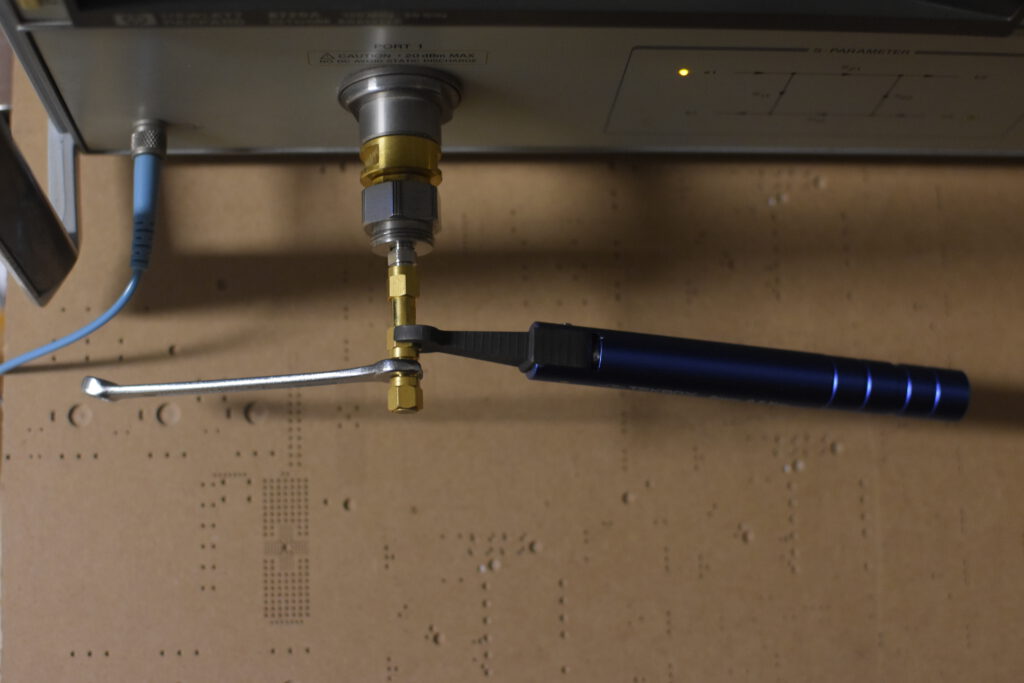
3.5mm precision connecters not only offer – usually – better microwave frequency capability but also better mating repeatability due to their construction. These types of connectors do not use a dielectric/foam insulator, but air.
Even better connectors are either slotless are rimmed slotted sockets. Also the amount of slots has an influence on the repeatability.

Actual Measurements

But what’s all that uncertainty stuff anyhow ? What can we achieve with all these specifications added to the measurement ?

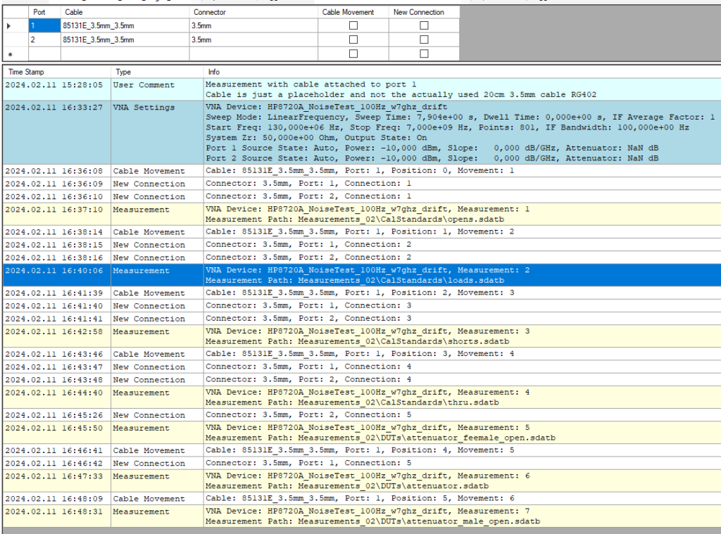
As depicted in the left image, it’s essential to log each measurement individually and conduct the calibration process on the PC side. Alongside specifying the connector type, it’s crucial to designate the cable utilized (I opted for an existing HP cable since, at the time of measurement, none of my cables had been characterized). With this information, METAS VNA Tools can effectively compute the uncertainty propagated throughout your measurement series.

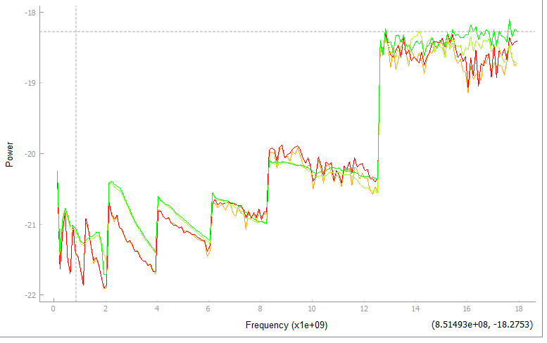
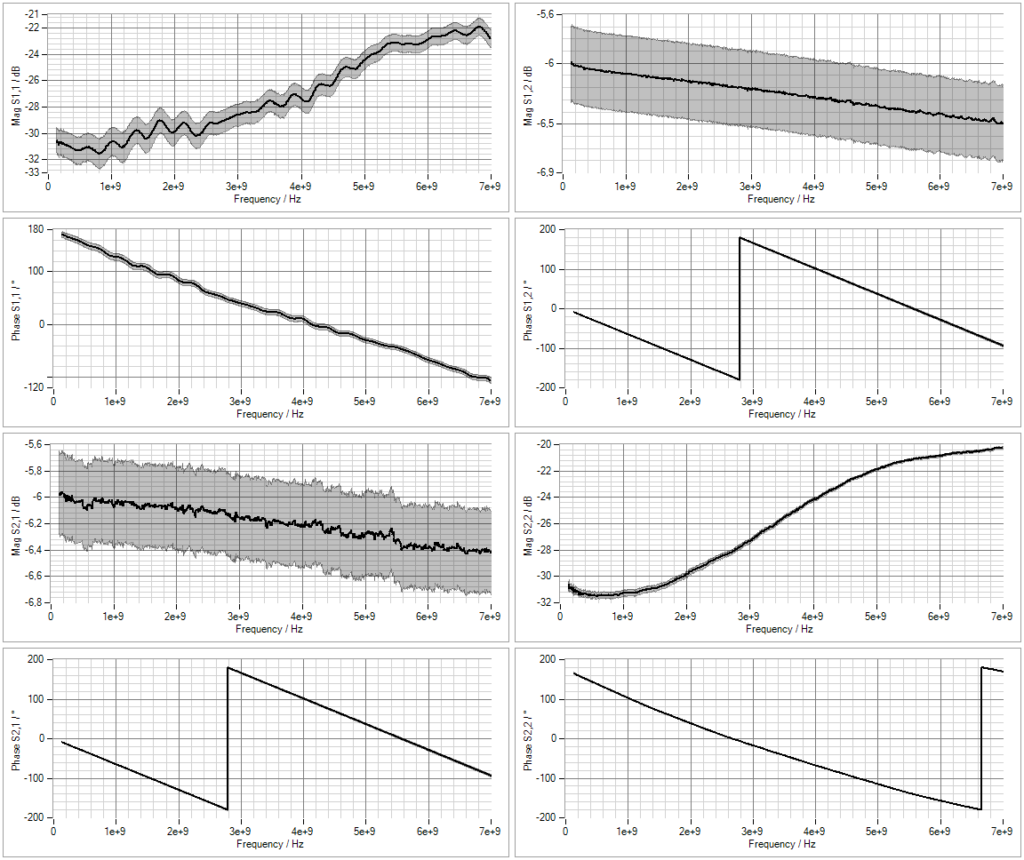
In the middle image, you’ll notice the likely range of your measurement result. Notably, one of the two transmission parameters exhibits significantly higher uncertainty. This can be attributed to the frequent movement of the cable connected to that port, between calibration measurements.

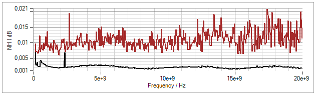
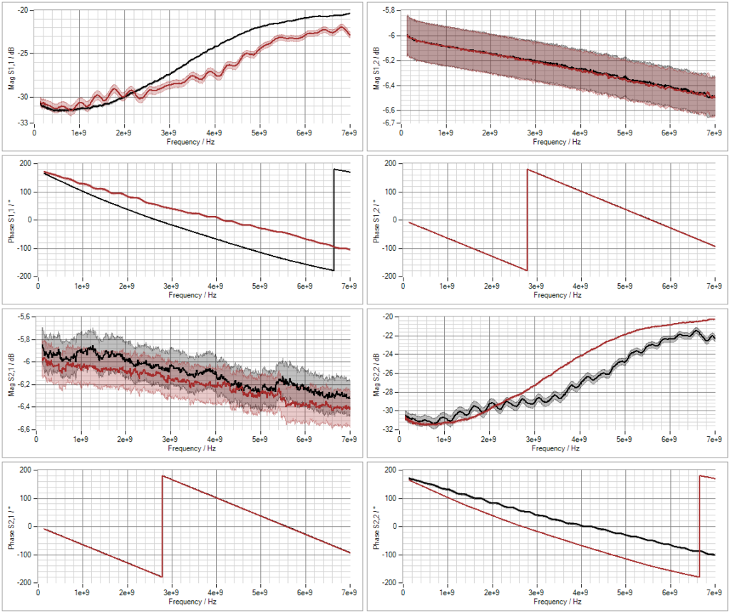
Regarding the peculiar behavior of the receiver for port 2, initial suspicions pointed towards issues with the calibration kit or similar factors. However, as illustrated in the rightmost image, the receiver for port 2 consistently displays a noisy trace, coupled with a poorer noise floor, regardless of the direction in which it’s oriented.

For clarity: The red trace represents the verification attenuator in the male-to-female orientation, while the black trace represents the female-to-male orientation. All S-Parameters are compared without altering their port configurations.

A general note or disclaimer regarding this article: Neither my VNA nor any other equipment in my modest electronics workshop has undergone calibration, nor would it be practical to pursue calibration standard tracing or similar procedures. However, despite this limitation, I find this topic to be quite intriguing. Moreover, I believe that hobbyists stand to gain valuable insights into the significance of their measurement results within a microwave environment through exploration of this discussion.